


What do the digits of pi, colliding blocks and quantum search algorithms have in common? More than you might expect. Two playful papers, one from 2003 and one from December of 2019, provide the links between them. Together, they connect the worlds of dynamics, geometry and quantum computation, highlighting how even the most abstract math puzzles can have surprising physical relevance.
Block It Out
To begin understanding these connections, first imagine two metal blocks, each weighing 1 kilogram. They sit on a frictionless surface, with an immovable wall to their left. The one closer to the wall is stationary, but the second is sliding toward it from the right. A series of crashes is imminent, and with each collision, let’s assume no kinetic energy is lost. Under these ideal conditions, the process would unfold something like this:
The right block hits the left, transferring all of its momentum. The left block then bounces off the wall, returning to the right block for a third collision and another complete transfer of momentum.
Increase the mass of that right block, however, and things get more interesting. If it weighs 100 kilograms, it only transfers a small portion of its momentum to the small block with each collision, and instead of three bounces the turnaround results in 31.
At a mass ratio of 10,000-to-1, it takes 314 collisions before they’re all done.
Keep increasing the ratio in powers of 100 and you’ll see a shocking trend develop: The number of collisions will more closely approximate the digits of pi.
Gregory Galperin, a mathematician at Eastern Illinois University, was the first to notice this phenomenon. He explained it in 2003 by visualizing the motions of the blocks as a moving point, whose x-coordinate represents where one block is, and whose y-coordinate represents where the second block is. The way this point moves around in the xy-plane is related to a half-circle, thus bringing pi into the picture.
It’s a remarkable result, even if those ideal conditions make it seem useless. In math, though, brushing aside the messiness of the real world can uncover a pure pattern that reveals unexpected connections to other fields.
Early in 2019, I published a set of three videos about Galperin’s result, and among the viewers was Adam Brown, a researcher at Google and a physicist at Stanford University. At a conference several months later, he pulled me aside to share an observation. To his delight, he’d discovered that the math explaining these block dynamics, if viewed the right way, is actually identical to the math explaining one of the most famous quantum algorithms.
A Quantum Approach
This brings us to the second piece of the puzzle: how quantum searches work.
Suppose you have a long list of unsorted names—say a million of them—and you want to find a particular one. There’s nothing you can do except check each name, one by one, until you find it. On average, this will take half a million steps. Sometimes it’ll be more, sometimes less, but you’re definitely in for a long day.
A computer could tackle this search for you, but for bigger unsorted lists, the amount of time it takes will grow in proportion to the size of the list. At least, that’s true for a classical computer. But in 1996, Lov Grover, then at Bell Labs, described how a quantum computer can perform the search much faster, in less than 1,000 steps. More generally, for a list of size N, a quantum computer could handle it with about π/4 square root of N steps. Note that as N grows, this runtime for a quantum computer grows more slowly than it would for a classical computer.
Such an efficient search is possible because a quantum computer acts on every element of the list simultaneously. However, it’s not simply doing everything a classical computer would do, just all at the same time.
A classical computer answers the question: “Is the 21st element of the list the name I’m looking for?” And so on for every other position on the list between 0 and 999,999. Straightforward, but not very efficient.
By contrast, the way Grover’s algorithm treats the list looks bizarre at first but ultimately proves more useful. With a classical computer, you can simply read bits out of memory; in quantum computation, the uncertainties involved mean you can’t directly pull up the components of a vector you’re working with. Instead, each position on the list carries the additional structure of a probability value. Rather than seeing what name is at a given position, you perform a measurement of the full list which returns a random position—called an index—according to these probabilities. For reasons having to do with the underlying quantum mechanics, instead of working with the probability values directly, we work with numbers whose square corresponds to the probability of getting the index that the name corresponds to.
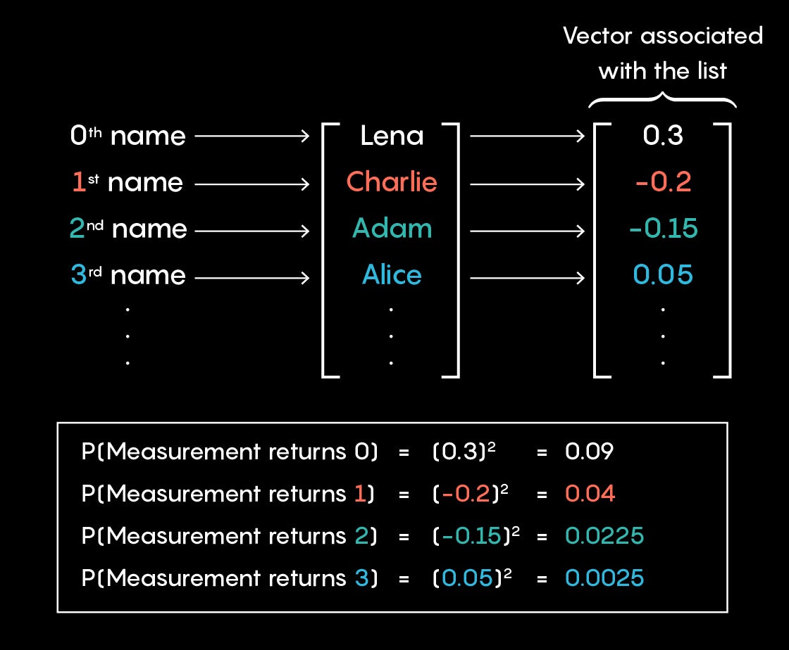
How can reading a random index possibly be useful? The art of quantum computation is to manipulate this list of probabilities so that the odds work for you. In our example, that means figuring out some way (which is what Grover’s algorithm does) to get the number associated with the index of the name you’re looking for to be close to 1, while all others are close to 0. That way, when you take a reading of this list and get back an index, you’ll know with a high probability that this is the one with the name you’re looking for.
The tools of quantum computation consist of the operations a researcher can perform on this list of probabilities. In math, such a list of numbers is called a vector. It’s often helpful to think of a vector as a point in coordinate space, or as an arrow drawn from the origin to this point.
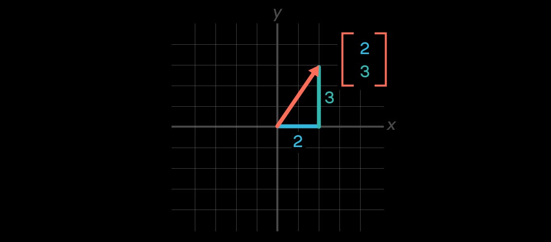
A vector with two components is pictured as an arrow in two-dimensional space. One with 1,000,000 components lives in a mind-boggling 1,000,000-dimensional space. The operations a quantum computer performs look like flips and rotations to this arrow. Numerically, each operation is represented by a matrix.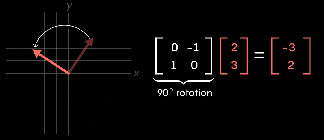
Quantum computation is extra speedy because each operation acts on the full vector of probabilities in one fell swoop, rather than going component by component. Grover discovered a clever way to manipulate a given vector with a pair of alternating operations that result in a vector with the probabilities we want. Importantly, the total number of operations required is much smaller than the size of the list.
If you’re having trouble picturing how this might work, you’re not alone. That’s why Adam Brown was so excited to find a way to think about these abstract vector manipulations in terms of a more tangible puzzle.
Hidden Connections
Brown happened to have Grover’s algorithm on his mind when he saw my videos outlining how colliding blocks compute pi, and he spotted a connection. “If you’ve spent the day thinking about quantum search, everything starts to look like quantum search,” Brown said, “which was fortuitous because in this case it really was quantum search.”
While Galperin’s original paper on the block collisions used a space that encodes the positions of each block, the connection to Grover’s quantum search starts instead with a vector whose x and y components encode the velocity of each block. Each collision between the blocks results in a certain operation to this vector, a change to the components. For example, when the left block hits the wall and reverses direction, it means the y component of our vector gets multiplied by −1, while the x component remains unchanged. Geometrically, this looks like a flip about the x-axis.
Similarly, when the two blocks hit each other, the way their velocities change looks like another flip of this vector, this one a little off-center. Play the scenario out, and the left block hits the wall again, meaning another x-axis flip. Then another block-block collision means another off-center flip. Eventually, given enough collisions, the vectors fill in a familiar shape: a circle.
Brown observed that if you frame the setup appropriately, these two operations going back and forth are identical to the two operations Grover used in his quantum search algorithm.
To understand how, think of the big block on the right as many 1-kilogram blocks glued together. Then, instead of a two-dimensional vector describing each velocity, it would be an N-dimensional vector, where N is the total number of little blocks, including the isolated one on the left. Each of these little blocks will correspond to a name on the unsorted list, and the single block on the left represents the target name.
In his paper, Brown proved that the way these block collisions change the vector describing them is precisely the same as the way Grover’s algorithm changes a quantum vector representing an unsorted list of names. The moment in the block-colliding process when the big block is just about to turn around, and almost all the energy of the system is in the little block, corresponds to the moment in Grover’s algorithm when almost all of the probability lies with the name you want to find.
The fact that pi shows up when we count the collisions is mirrored in the runtime of Grover’s algorithm: π/4 square root of N steps. The square root in that expression also reflects how further digits of pi (in base 10) come from multiplying the mass of the big block by 100.
“At the moment it’s more of a curiosity,” Brown said. “But in physics, we have learned that the more ways we have to think about a problem, the more insight we can glean, so hopefully this will one day be useful. We don’t have many great alternative ways to visualize Grover’s [algorithm].”
These connections highlight the power of a universal mathematical language. Using vectors to encode the state of a physical system works just as well with macroscale block collisions as it does with microscale quantum states. Many fundamental ideas in math, which may at first seem frustratingly removed from reality, prove to be powerful tools because dropping the physical details from one field can reveal otherwise hidden connections to another.
All videos and in-article images, credit: Grant Sanderson (3Blue1Brown)
Lead image: Lucy Reading-Ikkanda/Quanta Magazine